Deep Learning vs Machine Learning

In this blog post Deep Learning vs Machine Learning Choosing the Right Approach we will unpack what each approach really means, where they shine, and how to make a confident choice for your next project. Whether you build models or fund them, the goal here is clarity and practical next steps.

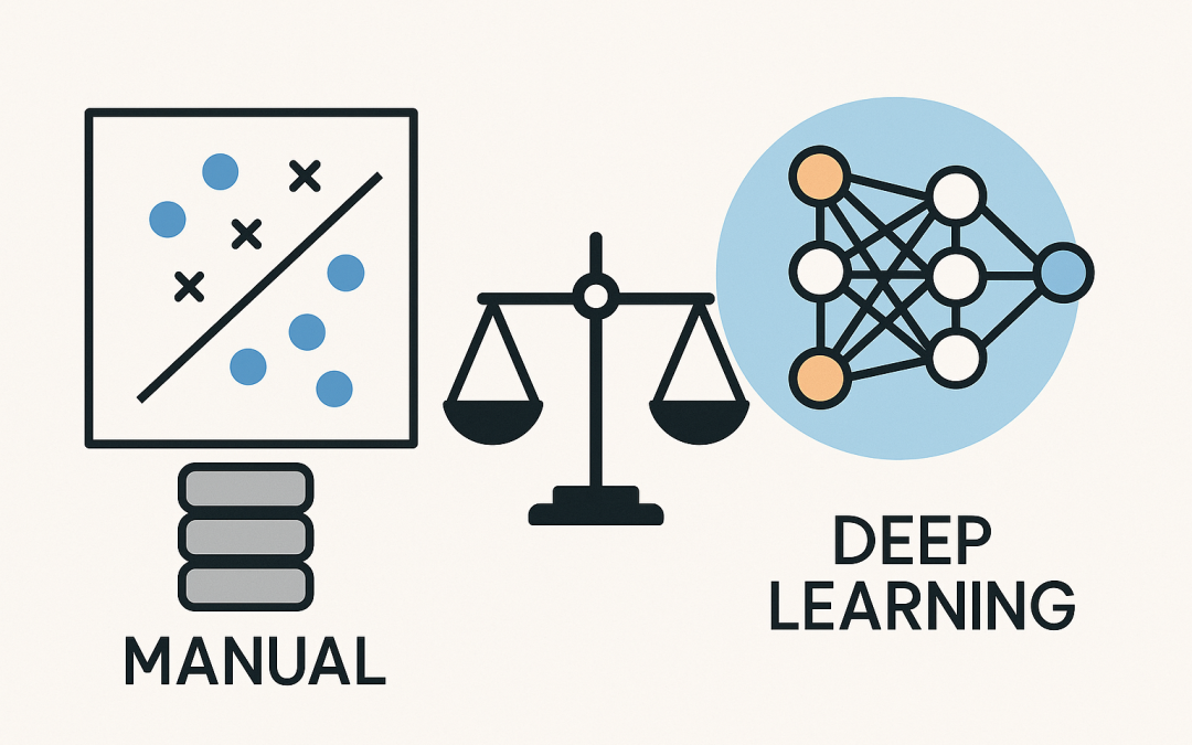
At a high level, machine learning (ML) covers a family of algorithms that learn patterns from data with human-crafted features. Deep learning (DL) is a subset of ML that uses multi-layer neural networks to learn the features and the predictor at the same time. ML tends to be faster to develop and easier to explain; DL tends to excel on complex, high-dimensional data like images, audio, and natural language—if you have the data and compute to match.

What machine learning actually is

Classical ML uses algorithms such as linear/logistic regression, decision trees, random forests, gradient boosting, and support vector machines. The key idea is separating feature engineering from model learning:

• You design features from raw data (e.g., ratios, counts, domain-specific transforms).
• The algorithm maps those features to predictions by minimizing a loss function.

Strengths:

• Great for structured/tabular data with limited rows (thousands to low millions).
• Faster to train and tune; strong baselines with minimal compute.
• Often more interpretable and easier to validate under governance.

Trade-offs:

• Feature engineering can be labor-intensive and brittle to distribution shifts.
• Performance can plateau on unstructured data or very complex relationships.

What deep learning actually is

Deep learning uses neural networks with many layers, trained via backpropagation and stochastic gradient descent. Each layer transforms inputs to increasingly abstract representations—automating feature learning. Architectures include CNNs for vision, RNNs/Transformers for sequences and language, and MLPs for tabular data when large datasets exist.

Strengths:

• State-of-the-art performance on unstructured data and complex patterns.
• End-to-end learning reduces manual feature engineering.
• Pretrained models and transfer learning cut data and compute needs.

Trade-offs:

• Needs more data, more compute (often GPUs), and careful training.
• Harder to explain and debug; longer iteration cycles.
• Operational overhead for serving large models with low latency.

How they learn under the hood

• Representation: ML relies on human-designed features; DL learns representations automatically via layers and nonlinear activations (ReLU, GELU).
• Optimization: Both minimize a loss; DL uses gradient-based updates over millions to billions of parameters; ML often optimizes fewer parameters or uses tree splits.
• Capacity and regularization: DL has high capacity; needs dropout, weight decay, data augmentation, and early stopping. ML uses regularization (L1/L2), tree depth limits, and shrinkage.
• Scale: DL benefits greatly from large datasets and parallel compute; ML saturates sooner and is efficient on CPUs.
• Inference: DL may require GPUs or model compression for real-time SLAs; ML is typically CPU-friendly with lower memory footprints.

When to choose which

• Data type: Tabular/relational with dozens to hundreds of columns → start with ML. Images, audio, text, time-series with complex temporal patterns → DL or pretrained DL.
• Data volume: Small datasets (≤50k rows) → ML usually wins. Large datasets or access to high-quality labels → DL gains advantage.
• Explainability: Regulated decisions (credit, healthcare) → ML or explainable DL with strong post-hoc techniques.
• Latency and cost: Tight budgets or strict millisecond SLAs → ML or compressed DL (quantization, distillation).
• Iteration speed: Need quick cycles and A/Bs → ML baseline first, then layered DL experiments.

Minimal code comparison

Two tiny examples for a binary classification problem. One with scikit-learn (ML), one with PyTorch (DL). They are intentionally short and omit production concerns.

Classical ML with scikit-learn

from sklearn.datasets import make_classification
from sklearn.model_selection import train_test_split
from sklearn.ensemble import RandomForestClassifier
from sklearn.metrics import roc_auc_score

X, y = make_classification(n_samples=5000, n_features=20, random_state=42)
X_train, X_test, y_train, y_test = train_test_split(X, y, test_size=0.2, random_state=42)

model = RandomForestClassifier(n_estimators=200, max_depth=8, random_state=42)
model.fit(X_train, y_train)
print("AUC:", roc_auc_score(y_test, model.predict_proba(X_test)[:,1]))

Deep learning with PyTorch

import torch
import torch.nn as nn
from sklearn.datasets import make_classification
from sklearn.model_selection import train_test_split
from sklearn.preprocessing import StandardScaler
from sklearn.metrics import roc_auc_score

# Data
X, y = make_classification(n_samples=5000, n_features=20, random_state=42)
X_train, X_test, y_train, y_test = train_test_split(X, y, test_size=0.2, random_state=42)
scaler = StandardScaler().fit(X_train)
X_train, X_test = scaler.transform(X_train), scaler.transform(X_test)

# Tensors
X_train = torch.tensor(X_train, dtype=torch.float32)
y_train = torch.tensor(y_train, dtype=torch.float32).unsqueeze(1)
X_test  = torch.tensor(X_test,  dtype=torch.float32)

device = torch.device("cuda" if torch.cuda.is_available() else "cpu")
X_train, y_train, X_test = X_train.to(device), y_train.to(device), X_test.to(device)

# Simple MLP
model = nn.Sequential(
    nn.Linear(20, 64), nn.ReLU(),
    nn.Linear(64, 32), nn.ReLU(),
    nn.Linear(32, 1), nn.Sigmoid()
).to(device)

opt = torch.optim.Adam(model.parameters(), lr=1e-3)
loss_fn = nn.BCELoss()

for epoch in range(10):
    opt.zero_grad()
    pred = model(X_train)
    loss = loss_fn(pred, y_train)
    loss.backward()
    opt.step()

with torch.no_grad():
    scores = model(X_test).cpu().numpy().ravel()

print("AUC:", roc_auc_score(y_test, scores))

For tabular tasks like this, the Random Forest often matches or beats the simple MLP with less tuning and compute. Swap in images or text, and DL typically pulls ahead—especially with transfer learning.

Architecture patterns on cloud

• Data layer: Object storage and data lakehouse for raw data; a feature store for curated signals.
• Training: Managed training jobs; CPU nodes for ML, GPU nodes for DL. Use spot/preemptible where safe.
• Experiment tracking: Centralized runs, metrics, and artifacts for reproducibility.
• Model registry: Versioned models with metadata, approvals, and rollout stages.
• Serving: Low-latency CPU endpoints for ML; autoscaled GPU or optimized CPU with quantized DL models.
• Monitoring: Data drift, concept drift, latency, and cost per prediction dashboards.

Cost and performance tips

• Always build a strong ML baseline first; it sets a realistic target and controls scope.
• Leverage pretrained DL models and fine-tune; it cuts data needs and compute by orders of magnitude.
• Use mixed precision on GPUs, gradient accumulation, and early stopping to save time and money.
• Compress models for production: quantization, pruning, and knowledge distillation.
• Batch offline predictions where latency is flexible; reserve real-time for what truly needs it.

Common pitfalls to avoid

• Data leakage from future or target-related features inflates offline scores and implodes in production.
• Overfitting due to insufficient regularization, augmentation, or cross-validation rigor.
• Unbalanced labels without proper metrics (AUC, F1, PR AUC) or calibrated thresholds.
• Poor reproducibility: missing seeds, untracked code/data versions, and ad hoc environments.
• Ignoring inference costs until late; a great model that is too expensive per request is not great.

A pragmatic adoption path

• Define the decision and metric that matters (AUC, RMSE, latency, cost per 1k predictions).
• Start with an ML baseline and a simple feature pipeline; instrument drift and cost metrics from day one.
• If the baseline ceiling is clear or the data is unstructured, evaluate a pretrained DL approach.
• Run side-by-side offline and online tests; monitor business impact, not just ML metrics.
• Harden the winner with model compression, CI/CD, canary rollouts, and continuous monitoring.

Summary

Machine learning and deep learning are not rivals—they are tools. ML gives you speed, simplicity, and strong performance on structured problems. DL unlocks state-of-the-art results on complex, high-dimensional data, provided you can feed it with labels and compute. Use ML to move fast and learn; use DL when the problem, data, and resources justify the jump. With a solid baseline, disciplined experiments, and the right cloud architecture, you can have both velocity and accuracy.

• Simplifying Windows 10 Integration with Microsoft Intune Using a Deep Link
• Running PyTorch in Microsoft Azure Machine Learning
• Cypher Queries and RAG Technology Explained
• How to Create an Azure AI Language Account Using REST API
• What Are Cypher Queries