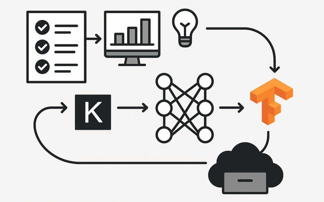
In this blog post Build a Keras Model for Real Projects From Idea to Deployment we will walk through a practical, end-to-end way to design, train, and ship a Keras model that stands up in real work.
Keras is a high-level deep learning API that runs on top of TensorFlow. It abstracts the heavy lifting—tensor math, automatic differentiation, and GPU acceleration—so you can focus on model architecture and data. Under the hood, TensorFlow builds a computational graph of layers and operations. During training, backpropagation adjusts the model’s parameters by computing gradients of a loss function and applying an optimizer like Adam. The result: concise code, strong performance, and production-grade tooling.
In Build a Keras Model for Real Projects From Idea to Deployment we’ll start with a clear, non-jargony overview of what matters, then move into code. We’ll cover data handling, architecture choices, training, evaluation, and deployment options—plus the small details that make a big difference when projects leave the notebook and head to production.
What you’ll build and why Keras
We’ll build a simple but real image classifier on the MNIST dataset to keep the code short and readable. The same pattern applies to tabular, text, or time series problems—you’ll swap the input pipeline and layers, but the workflow stays consistent.
- Keras keeps code compact and readable
- TensorFlow provides performance, distribution strategies, and serving
- Callbacks, metrics, and standardized saving make production easier
Set up and plan
Environment
# Install (CPU). For GPU, install tensorflow with appropriate CUDA/CuDNN.
pip install tensorflow
import os, random
import numpy as np
import tensorflow as tf

# Reproducibility (helps debugging and comparisons)
SEED = 42
random.seed(SEED)
np.random.seed(SEED)
tf.random.set_seed(SEED)
print(tf.__version__)
Define the objective and metric
- Objective: classify handwritten digits
- Primary metric: accuracy
- Secondary metric: validation loss (for early stopping)
Load and prepare data
We’ll use MNIST for clarity. In production, expect to spend more time here than anywhere else.
from tensorflow import keras

# Load data
(x_train, y_train), (x_test, y_test) = keras.datasets.mnist.load_data()

# Hold out a validation set from the training data
val_size = 10_000
x_val, y_val = x_train[-val_size:], y_train[-val_size:]
x_train, y_train = x_train[:-val_size], y_train[:-val_size]

# Normalize and add channel dimension
x_train = (x_train[..., np.newaxis] / 255.).astype("float32")
x_val   = (x_val[...,   np.newaxis] / 255.).astype("float32")
x_test  = (x_test[...,  np.newaxis] / 255.).astype("float32")

# Build performant tf.data pipelines
BATCH = 128
train_ds = (tf.data.Dataset.from_tensor_slices((x_train, y_train))
            .shuffle(10_000, seed=SEED)
            .batch(BATCH)
            .prefetch(tf.data.AUTOTUNE))
val_ds   = (tf.data.Dataset.from_tensor_slices((x_val, y_val))
            .batch(BATCH)
            .prefetch(tf.data.AUTOTUNE))
test_ds  = (tf.data.Dataset.from_tensor_slices((x_test, y_test))
            .batch(BATCH)
            .prefetch(tf.data.AUTOTUNE))
Build the Keras model
You can use the Sequential API for straightforward stacks, or the Functional API for more complex graphs (multiple inputs/outputs, skip connections). Let’s start with Sequential.
from tensorflow.keras import layers, models

model = models.Sequential([
    layers.Input(shape=(28, 28, 1)),
    layers.Conv2D(32, 3, activation="relu"),
    layers.Conv2D(64, 3, activation="relu"),
    layers.MaxPooling2D(),
    layers.Dropout(0.25),
    layers.Flatten(),
    layers.Dense(128, activation="relu"),
    layers.Dropout(0.5),
    layers.Dense(10, activation="softmax")
])

model.summary()
Compile with loss, optimizer, and metrics
model.compile(
    optimizer=keras.optimizers.Adam(learning_rate=1e-3),
    loss=keras.losses.SparseCategoricalCrossentropy(),
    metrics=["accuracy"]
)
Train with callbacks
Callbacks automate good hygiene—stop early when performance plateaus, lower the learning rate, and keep the best weights.
callbacks = [
    keras.callbacks.EarlyStopping(monitor="val_loss", patience=3, restore_best_weights=True),
    keras.callbacks.ReduceLROnPlateau(monitor="val_loss", factor=0.5, patience=2),
    keras.callbacks.ModelCheckpoint("mnist_cnn.keras", save_best_only=True)
]

history = model.fit(
    train_ds,
    validation_data=val_ds,
    epochs=20,
    callbacks=callbacks
)
Evaluate and predict
test_loss, test_acc = model.evaluate(test_ds)
print({"test_loss": float(test_loss), "test_acc": float(test_acc)})

# Predict a single sample
sample = x_test[:1]
p = model.predict(sample)
print("Predicted class:", int(np.argmax(p, axis=1)[0]))
Save and deploy
You have two common options: the native Keras format for portability, or TensorFlow SavedModel for serving. Use what your deployment target expects.
# Save in native Keras format (recommended for Keras 3 and most workflows)
model.save("mnist_cnn.keras")
reloaded = keras.models.load_model("mnist_cnn.keras")

# Save as TensorFlow SavedModel (useful for TF Serving)
keras.models.save_model(model, "export/mnist_savedmodel")

# Optional: Convert to TensorFlow Lite for mobile/edge
converter = tf.lite.TFLiteConverter.from_saved_model("export/mnist_savedmodel")
tflite_model = converter.convert()
with open("mnist.tflite", "wb") as f:
    f.write(tflite_model)
When to use the Functional API
For non-linear topologies, multiple inputs, or custom heads, switch to Functional. It is equally concise and far more flexible.
inputs = keras.Input(shape=(28, 28, 1))
x = layers.Conv2D(32, 3, activation="relu")(inputs)
x = layers.Conv2D(64, 3, activation="relu")(x)
x = layers.MaxPooling2D()(x)
x = layers.Flatten()(x)
branch = layers.Dense(64, activation="relu")(x)
class_logits = layers.Dense(10, activation="softmax", name="class_output")(branch)

func_model = keras.Model(inputs=inputs, outputs=class_logits)
func_model.compile(optimizer="adam", loss="sparse_categorical_crossentropy", metrics=["accuracy"])
Performance tips that matter
- Use tf.data with batch, map, cache, and prefetch to keep the GPU fed.
- Start with Adam and a small learning rate; adjust with ReduceLROnPlateau.
- Enable mixed precision on modern GPUs for speedups:
from tensorflow.keras import mixed_precision
mixed_precision.set_global_policy("mixed_float16")
# If you do this, set the final Dense layer dtype="float32" to avoid numeric issues.
- Scale out with MirroredStrategy for multi-GPU on one machine:
strategy = tf.distribute.MirroredStrategy()
with strategy.scope():
    # build and compile model here
    pass
- Profile a single epoch to find input bottlenecks before buying bigger GPUs.
Common pitfalls and how to fix them
- Overfitting: add Dropout, use data augmentation, or collect more data. Monitor val_loss.
- Underfitting: increase model capacity, train longer, or raise learning rate slightly.
- Data leakage: strict train/val/test separation, no peeking.
- Unstable training: normalize inputs, check labels, reduce learning rate.
- Inconsistent results: set seeds and avoid mixing old checkpoints with new code.
Adapting this to your domain
- Images: swap MNIST for your dataset; add data augmentation (RandomFlip, RandomRotation).
- Tabular: replace Conv2D with Dense stacks; use normalization and feature engineering.
- Text: use Embedding + LSTM/GRU or Transformers from KerasNLP.
- Time series: 1D Conv, LSTM/GRU, or Temporal Convolutional Networks.
Production checklists
- Version data, code, and models together; log metrics and hashes.
- Export a stable inference artifact (.keras or SavedModel) and keep an input schema.
- Add health checks and canary rollouts; monitor drift and performance in production.
- Retrain on a schedule or when drift exceeds a threshold.
Wrap up
Building with Keras is fast, readable, and production-ready when paired with TensorFlow’s tooling. Define the goal, get the data right, keep the model simple first, and automate the boring-but-critical parts with callbacks and standardized saves. With these patterns, you can move from prototype to deployment confidently—and repeatably—for your next computer vision, NLP, or tabular ML project.
